One of the reason why I often use INLA is because it allows for correlated random effects. In this blog post, I will handle random effect with temporal autocorrelation. INLA has several options for this. There are two major types of model, the first handles discrete time step, the latter continuous time steps.
Dummy data set
This blog post was inspired by a post on the R-Sig-Mixed models mailing list. Therefore I created some example data relevant for that post. The set-up were 34 participants received five random prompts per day for six weeks, asking them whether they were craving a particular drug.
The chunk below sets the design. Timestamp assumes that the participant were only prompted between 8:00 and 22:00. Hour are the timestamps rounded to the hour.
library(tidyverse)
── Attaching core tidyverse packages ──────────────────────── tidyverse 2.0.0 ──
✔ dplyr 1.1.2 ✔ readr 2.1.4
✔ forcats 1.0.0 ✔ stringr 1.5.0
✔ ggplot2 3.4.2 ✔ tibble 3.2.1
✔ lubridate 1.9.2.9000 ✔ tidyr 1.3.0
✔ purrr 1.0.1
── Conflicts ────────────────────────────────────────── tidyverse_conflicts() ──
✖ dplyr::filter() masks stats::filter()
✖ dplyr::lag() masks stats::lag()
ℹ Use the conflicted package (<http://conflicted.r-lib.org/>) to force all conflicts to become errors
set.seed(20180305)n_id <-34n_day <-7*6n_prompt <-5expand.grid(ID =seq_len(n_id),Day =seq_len(n_day),Prompt =seq_len(n_prompt)) %>%mutate(Timestamp =runif(n(), min =8, max =21.99999),Timestamp2 =round(Timestamp, 2),Hour =floor(Timestamp) ) -> example
Next we need to create a true model. Let’s assume a first order random walking along Timestamp and a random intercept per participant (Figure 1). A real life model would be more complicated. Choosing a simpler model keeps the computation time down.
So the current value is the average of the next and the previous value minus half of \(\Delta ^2 x_i\)
restrictions
\(\Delta^2 x_i \sim \mathcal{N}(0, \tau^{-1})\)
\(\sum \Delta x_i = 0\)
Fitting the models
We are using the defaults priors, except for the rw1 model where we use the currently recommended prior, which is not the default prior. We fitted the ar1 model once without sum-to-zero constraint (default) and once with sum-to-zero constraint.
library(INLA)model_ar1 <-inla( Craving ~f(Hour, model ="ar1") +f(ID, model ="iid"),family ="binomial", data = example, control.compute =list(waic =TRUE))
model_ar1c <-inla( Craving ~f(Hour, model ="ar1", constr =TRUE) +f(ID, model ="iid"),family ="binomial", data = example, control.compute =list(waic =TRUE))
pc_prec <-list(theta =list(prior ="pc.prec", param =c(0.5, 0.01)))model_rw1 <-inla( Craving ~f(Hour, model ="rw1", hyper = pc_prec) +f(ID, model ="iid"),family ="binomial", data = example, control.compute =list(waic =TRUE))
model_rw2 <-inla( Craving ~f(Hour, model ="rw2") +f(ID, model ="iid"),family ="binomial", data = example, control.compute =list(waic =TRUE))
Comparing the models
The fitted values for the models are very similar (Figure 2). The main difference is that the rw2 model is much smoother than the other models. The fitted values for the ar1 and rw1 model are very similar.
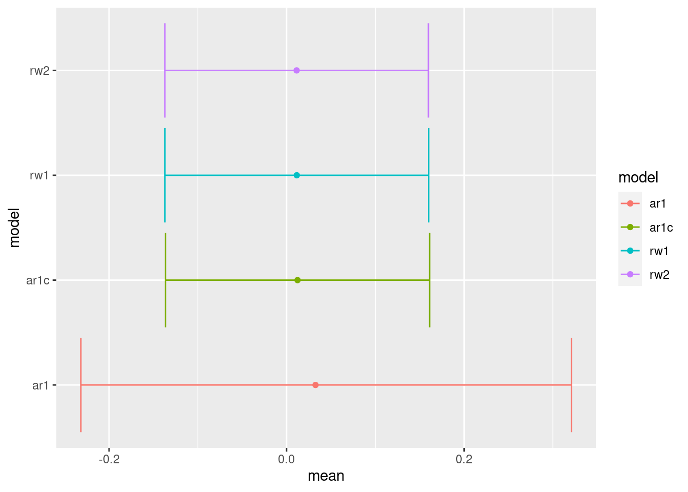
Figure 3 show the effect of the random effect of Hour under the different models. Overall, the pattern are very similar to those of the fitted values. This is expected since, besides the temporal pattern of Hour, the models only contains random intercepts. Note that uses the original scale, whereas Figure 3 uses the logit scale.
The default ar1 model has a much larger uncertainty than rw1 for both the random effect of Hour and the fixed intercept and yet the uncertainty for the fitted values is nearly identical for both models. This is because the default ar1 has no sum-to-zero constraint which makes the intercept unidentifiable when there is only one replica of the ar1 model. When the sum-to-zero constraint it also added to the ar1 model, then the results are very similar to those from the rw1 model.
binning the continuous time stamps in a large number of equally spaces bins allows to apply rw1 (also ar1 and rw2)
Fitting the models
The Timestamp was split in 100 groups for the crw2 model. We fitted the ou model both with and without sum-to-zero constraint. The time stamp was rounded to 0.01 hours for the rw1 model.
model_crw2 <-inla( Craving ~f(inla.group(Timestamp, n =100), model ="crw2") +f(ID, model ="iid"),family ="binomial", data = example, control.compute =list(waic =TRUE))
model_ou <-inla( Craving ~f(Timestamp, model ="ou") +f(ID, model ="iid"),family ="binomial", data = example, control.compute =list(waic =TRUE))
model_ouc <-inla( Craving ~f(Timestamp, model ="ou", constr =TRUE) +f(ID, model ="iid"),family ="binomial", data = example, control.compute =list(waic =TRUE))
model_rw1t <-inla( Craving ~f(Timestamp2, model ="rw1", hyper = pc_prec) +f(ID, model ="iid"),family ="binomial", data = example, control.compute =list(waic =TRUE))
Comparing the models
The fitted values in Figure 5 are more fine grained than those in Figure 2, simply because we use more fine grained time information. The crw2 model generates a rather smooth pattern. The rw1 model produces similar patterns that the ou model, although the ou seems to be a bit more extreme than the rw1 model. The credible interval of ou, ouc and rw1 are very similar.
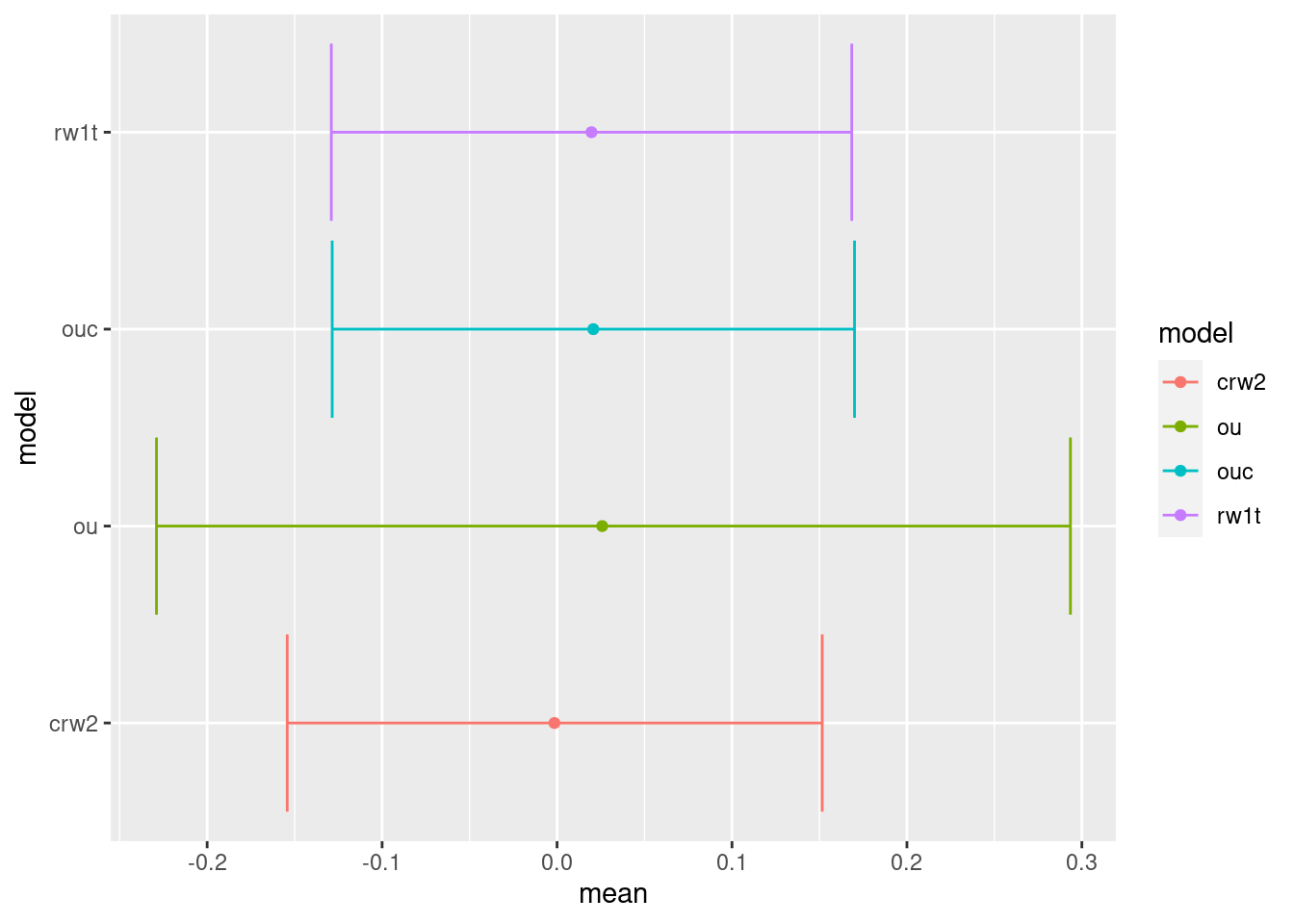
When we look at the random effects (Figure 6) and the fixed effects (Figure 7), we can draw similar conclusions as from Figure 3 and Figure 7: the ou without sum-to-zero constraint has wider credible intervals. Adding the sum-to-zero constrains to ou shrinks the credible intervals, although they remain wide than those for rw1.
Figure 7: Comparison of the fixed effects of the different continuous time step models
The ou model and the rw1 model on the fine grained time stamps have the lowest \(WAIC\). Note that the data was generated using an rw1 model at this fine grained level.
Each fitted inla object contains information on the time that was used to fit the model. It is interesting to see that with this example the ar1 model is much faster than the rw1 model with similar detail (on Hour). Likewise is the ou model faster than the rw1 model (both on Timestamp). Applying the sum-to-zero constraint on ar1 and ou requires some extra time.