library(leaflet)
library(scales)
library(sf)
library(tidyverse)
goose <- readRDS("data/anser_fabalis_rossicus.rds")
set.seed(20180712)Comparing inlabru with INLA
statistics
mixed-models
inlabru is an R package which builds on top of the INLA package. I had the opportunity to take a workshop on it during the International Statistical Ecology Workshop ISEC2018 in St Andrews. This was a five day workshop condensed into a single day, hence the pace was very high. It gave us a good overview of the possibilities of inlabru but no time to try it on our own data. This is an updated version of the original post due to changes in the package used in the original post.
inlabru has two main functions: bru() and lgcp(). bru() is a wrapper for INLA::inla(). lgcp() is intended to fit log Gaussian Cox processes. I will focus on bru and compare it with INLA::inla() as I find that bru() makes things a lot easier.
Tundra bean goose
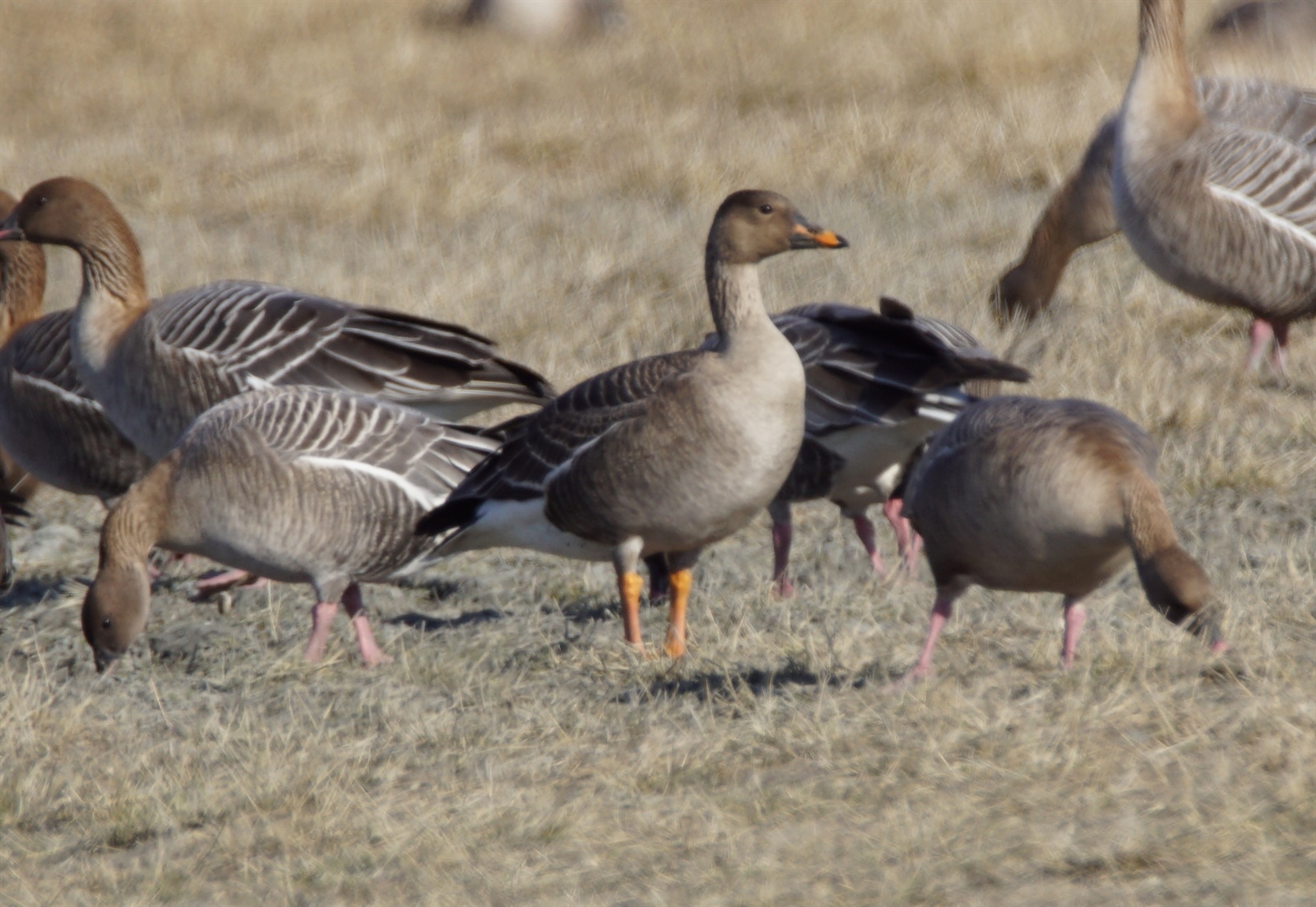
The test data is derived from the “Wintering waterbirds in Flanders, Belgium”, freely available at GBIF (https://doi.org/10.15468/lj0udq). I’ve extracted the observations from the tundra bean goose (Anser fabalis rossicus, Figure 1). The dataset was limited to those locations with at least 6 occurrences during at least 3 years. Months with lower number of count were removed. Figure 2 indicates the sum of all observed geese in the data. Note that these totals are somewhat misleading since there are a fair amount of missing observations (Figure 3). The geographic distribution of the data is given in Figure 4.


INLA vs inlabru
Fixed effects only
Let’s start with a very simple model with contains only the year centred to the last year. The syntax of both models is very similar. bru() is a bit shorted because it returns both \(WAIC\) and \(DIC\) by default. The models are identical because bru() is just a wrapper for inla(). Their summary output is somewhat different in terms of lay-out and which information is given.
library(INLA)
library(inlabru)
goose |>
mutate(cyear = .data$year - max(.data$year)) -> goose
m0_inla <- inla(
count ~ cyear, data = goose, family = "nbinomial",
control.compute = list(waic = TRUE, dic = TRUE)
)
m0_inlabru <- bru(count ~ cyear, data = goose, family = "nbinomial")
summary(m0_inla)
Call:
   c("inla.core(formula = formula, family = family, contrasts = contrasts,
   ", " data = data, quantiles = quantiles, E = E, offset = offset, ", "
   scale = scale, weights = weights, Ntrials = Ntrials, strata = strata,
   ", " lp.scale = lp.scale, link.covariates = link.covariates, verbose =
   verbose, ", " lincomb = lincomb, selection = selection, control.compute
   = control.compute, ", " control.predictor = control.predictor,
   control.family = control.family, ", " control.inla = control.inla,
   control.fixed = control.fixed, ", " control.mode = control.mode,
   control.expert = control.expert, ", " control.hazard = control.hazard,
   control.lincomb = control.lincomb, ", " control.update =
   control.update, control.lp.scale = control.lp.scale, ", "
   control.pardiso = control.pardiso, only.hyperparam = only.hyperparam,
   ", " inla.call = inla.call, inla.arg = inla.arg, num.threads =
   num.threads, ", " keep = keep, working.directory = working.directory,
   silent = silent, ", " inla.mode = inla.mode, safe = FALSE, debug =
   debug, .parent.frame = .parent.frame)" )
Time used:
    Pre = 0.803, Running = 1.05, Post = 0.029, Total = 1.88
Fixed effects:
             mean    sd 0.025quant 0.5quant 0.975quant  mode kld
(Intercept) 4.560 0.218      4.133    4.560      4.987 4.560   0
cyear       0.134 0.026      0.083    0.134      0.185 0.134   0

Model hyperparameters:
                                                        mean    sd 0.025quant
size for the nbinomial observations (1/overdispersion) 0.047 0.003      0.043
                                                       0.5quant 0.975quant
size for the nbinomial observations (1/overdispersion)    0.047      0.053
                                                        mode
size for the nbinomial observations (1/overdispersion) 0.047

Deviance Information Criterion (DIC) ...............: 5913.61
Deviance Information Criterion (DIC, saturated) ....: 823.50
Effective number of parameters .....................: 2.92

Watanabe-Akaike information criterion (WAIC) ...: 5914.06
Effective number of parameters .................: 3.18

Marginal log-Likelihood:  -3003.70
 is computed
Posterior summaries for the linear predictor and the fitted values are computed
(Posterior marginals needs also 'control.compute=list(return.marginals.predictor=TRUE)')summary(m0_inlabru)inlabru version: 2.8.0
INLA version: 23.06.29
Components:
cyear: main = linear(cyear), group = exchangeable(1L), replicate = iid(1L)
Intercept: main = linear(1), group = exchangeable(1L), replicate = iid(1L)
Likelihoods:
Family: 'nbinomial'
Data class: 'data.frame'
Predictor: count ~ .
Time used:
Pre = 0.596, Running = 1.36, Post = 0.0555, Total = 2.01
Fixed effects:
mean sd 0.025quant 0.5quant 0.975quant mode kld
cyear 0.134 0.026 0.083 0.134 0.185 0.134 0
Intercept 4.560 0.218 4.133 4.560 4.987 4.560 0
Model hyperparameters:
mean sd 0.025quant
size for the nbinomial observations (1/overdispersion) 0.047 0.003 0.043
0.5quant 0.975quant
size for the nbinomial observations (1/overdispersion) 0.047 0.053
mode
size for the nbinomial observations (1/overdispersion) 0.047
Deviance Information Criterion (DIC) ...............: 5913.61
Deviance Information Criterion (DIC, saturated) ....: 823.50
Effective number of parameters .....................: 2.92
Watanabe-Akaike information criterion (WAIC) ...: 5914.06
Effective number of parameters .................: 3.18
Marginal log-Likelihood: -3008.08
is computed
Posterior summaries for the linear predictor and the fitted values are computed
(Posterior marginals needs also 'control.compute=list(return.marginals.predictor=TRUE)')A drawback is that bru() doesn’t handle factor fixed effects. In a previous version it yielded a warning about invalid factor levels when fitting the model. Unfortunately you didn’t get the warning when getting the summary. You needed to be critical and noticed that the parameters of the model are not what you would expect. The current version throws a cryptic error. The workaround is to convert the factor variable into a set of dummy variables and use those. Creating the dummy variable is straight forward with model.matrix(). But adding them to the model is not very efficient when you have factor variables with more than a just few levels.
m1_inla <- inla(
  count ~ cyear + month, data = goose, family = "nbinomial",
  control.compute = list(waic = TRUE, dic = TRUE)
)
m1_inlabru <- bru(count ~ cyear + month, data = goose, family = "nbinomial")
Error in validObject(r): invalid class "dgTMatrix" object: 'x' slot is not of type "double"summary(m1_inla)
Call:
   c("inla.core(formula = formula, family = family, contrasts = contrasts,
   ", " data = data, quantiles = quantiles, E = E, offset = offset, ", "
   scale = scale, weights = weights, Ntrials = Ntrials, strata = strata,
   ", " lp.scale = lp.scale, link.covariates = link.covariates, verbose =
   verbose, ", " lincomb = lincomb, selection = selection, control.compute
   = control.compute, ", " control.predictor = control.predictor,
   control.family = control.family, ", " control.inla = control.inla,
   control.fixed = control.fixed, ", " control.mode = control.mode,
   control.expert = control.expert, ", " control.hazard = control.hazard,
   control.lincomb = control.lincomb, ", " control.update =
   control.update, control.lp.scale = control.lp.scale, ", "
   control.pardiso = control.pardiso, only.hyperparam = only.hyperparam,
   ", " inla.call = inla.call, inla.arg = inla.arg, num.threads =
   num.threads, ", " keep = keep, working.directory = working.directory,
   silent = silent, ", " inla.mode = inla.mode, safe = FALSE, debug =
   debug, .parent.frame = .parent.frame)" )
Time used:
    Pre = 0.531, Running = 0.776, Post = 0.0306, Total = 1.34
Fixed effects:
             mean    sd 0.025quant 0.5quant 0.975quant  mode kld
(Intercept) 2.704 0.259      2.195    2.704      3.213 2.704   0
cyear       0.177 0.026      0.127    0.177      0.227 0.177   0
monthdec    2.116 0.337      1.456    2.116      2.777 2.116   0
monthjan    2.760 0.343      2.087    2.760      3.434 2.760   0
monthfeb    2.353 0.332      1.703    2.353      3.003 2.353   0

Model hyperparameters:
                                                        mean    sd 0.025quant
size for the nbinomial observations (1/overdispersion) 0.051 0.003      0.046
                                                       0.5quant 0.975quant
size for the nbinomial observations (1/overdispersion)    0.051      0.057
                                                        mode
size for the nbinomial observations (1/overdispersion) 0.051

Deviance Information Criterion (DIC) ...............: 5870.18
Deviance Information Criterion (DIC, saturated) ....: 827.88
Effective number of parameters .....................: 5.86

Watanabe-Akaike information criterion (WAIC) ...: 5871.70
Effective number of parameters .................: 6.64

Marginal log-Likelihood:  -2991.55
 is computed
Posterior summaries for the linear predictor and the fitted values are computed
(Posterior marginals needs also 'control.compute=list(return.marginals.predictor=TRUE)')
goose |>
model.matrix(object = ~month) |>
as.data.frame() |>
select(-1) |>
bind_cols(goose) -> goose
m1_inlabru <- bru(
count ~ cyear + monthdec + monthjan + monthfeb, data = goose,
family = "nbinomial"
)
summary(m1_inlabru)inlabru version: 2.8.0
INLA version: 23.06.29
Components:
cyear: main = linear(cyear), group = exchangeable(1L), replicate = iid(1L)
monthdec: main = linear(monthdec), group = exchangeable(1L), replicate = iid(1L)
monthjan: main = linear(monthjan), group = exchangeable(1L), replicate = iid(1L)
monthfeb: main = linear(monthfeb), group = exchangeable(1L), replicate = iid(1L)
Intercept: main = linear(1), group = exchangeable(1L), replicate = iid(1L)
Likelihoods:
Family: 'nbinomial'
Data class: 'data.frame'
Predictor: count ~ .
Time used:
Pre = 0.488, Running = 1.23, Post = 0.0697, Total = 1.79
Fixed effects:
mean sd 0.025quant 0.5quant 0.975quant mode kld
cyear 0.177 0.026 0.127 0.177 0.227 0.177 0
monthdec 2.117 0.337 1.456 2.117 2.777 2.117 0
monthjan 2.760 0.343 2.087 2.760 3.434 2.760 0
monthfeb 2.353 0.331 1.703 2.353 3.003 2.353 0
Intercept 2.704 0.259 2.195 2.704 3.213 2.704 0
Model hyperparameters:
mean sd 0.025quant
size for the nbinomial observations (1/overdispersion) 0.051 0.003 0.046
0.5quant 0.975quant
size for the nbinomial observations (1/overdispersion) 0.051 0.057
mode
size for the nbinomial observations (1/overdispersion) 0.051
Deviance Information Criterion (DIC) ...............: 5870.18
Deviance Information Criterion (DIC, saturated) ....: 827.87
Effective number of parameters .....................: 5.86
Watanabe-Akaike information criterion (WAIC) ...: 5871.70
Effective number of parameters .................: 6.64
Marginal log-Likelihood: -2995.93
is computed
Posterior summaries for the linear predictor and the fitted values are computed
(Posterior marginals needs also 'control.compute=list(return.marginals.predictor=TRUE)')Random effects
inla() use the f() function to specify the random effects. bru() is very liberal and allows the user to choose any name, as long as it is a valid function name. In the example below we use site. For more detail see help("bru.components"). The downside is that bru() requires integer coded levels which go from 1 to the number of levels. We use the as.integer(factor()) trick to get these indices. Furthermore you need to supply the number of levels in the random effect for some random effects models.
comp_inla <- count ~ cyear + month + f(location_id, model = "iid")
m2_inla <- inla(
  comp_inla, data = goose, family = "nbinomial",
  control.compute = list(waic = TRUE, dic = TRUE)
)
goose |>
  mutate(
    loc_id = factor(.data$location_id) |>
      as.integer()
  ) -> goose
n_loc <- max(goose$loc_id)
comp_inlabru <- count ~ cyear + monthdec + monthjan + monthfeb +
  site(main = loc_id, model = "iid", n = n_loc)
m2_inlabru <- bru(comp_inlabru, data = goose, family = "nbinomial")
summary(m2_inla)
Call:
   c("inla.core(formula = formula, family = family, contrasts = contrasts,
   ", " data = data, quantiles = quantiles, E = E, offset = offset, ", "
   scale = scale, weights = weights, Ntrials = Ntrials, strata = strata,
   ", " lp.scale = lp.scale, link.covariates = link.covariates, verbose =
   verbose, ", " lincomb = lincomb, selection = selection, control.compute
   = control.compute, ", " control.predictor = control.predictor,
   control.family = control.family, ", " control.inla = control.inla,
   control.fixed = control.fixed, ", " control.mode = control.mode,
   control.expert = control.expert, ", " control.hazard = control.hazard,
   control.lincomb = control.lincomb, ", " control.update =
   control.update, control.lp.scale = control.lp.scale, ", "
   control.pardiso = control.pardiso, only.hyperparam = only.hyperparam,
   ", " inla.call = inla.call, inla.arg = inla.arg, num.threads =
   num.threads, ", " keep = keep, working.directory = working.directory,
   silent = silent, ", " inla.mode = inla.mode, safe = FALSE, debug =
   debug, .parent.frame = .parent.frame)" )
Time used:
    Pre = 0.471, Running = 3.72, Post = 0.0411, Total = 4.23
Fixed effects:
             mean    sd 0.025quant 0.5quant 0.975quant  mode kld
(Intercept) 1.884 0.414      1.070    1.884      2.697 1.884   0
cyear       0.178 0.029      0.121    0.178      0.235 0.178   0
monthdec    1.690 0.353      0.997    1.690      2.383 1.690   0
monthjan    2.588 0.345      1.911    2.588      3.264 2.588   0
monthfeb    2.497 0.335      1.840    2.497      3.155 2.497   0

Random effects:
  Name    Model
    location_id IID model

Model hyperparameters:
                                                        mean    sd 0.025quant
size for the nbinomial observations (1/overdispersion) 0.064 0.004      0.057
Precision for location_id                              0.425 0.134      0.218
                                                       0.5quant 0.975quant
size for the nbinomial observations (1/overdispersion)    0.064      0.072
Precision for location_id                                 0.407      0.740
                                                        mode
size for the nbinomial observations (1/overdispersion) 0.064
Precision for location_id                              0.372

Deviance Information Criterion (DIC) ...............: 5747.06
Deviance Information Criterion (DIC, saturated) ....: 855.02
Effective number of parameters .....................: 27.50

Watanabe-Akaike information criterion (WAIC) ...: 5753.23
Effective number of parameters .................: 26.71

Marginal log-Likelihood:  -2955.38
 is computed
Posterior summaries for the linear predictor and the fitted values are computed
(Posterior marginals needs also 'control.compute=list(return.marginals.predictor=TRUE)')summary(m2_inlabru)inlabru version: 2.8.0
INLA version: 23.06.29
Components:
cyear: main = linear(cyear), group = exchangeable(1L), replicate = iid(1L)
monthdec: main = linear(monthdec), group = exchangeable(1L), replicate = iid(1L)
monthjan: main = linear(monthjan), group = exchangeable(1L), replicate = iid(1L)
monthfeb: main = linear(monthfeb), group = exchangeable(1L), replicate = iid(1L)
site: main = iid(loc_id), group = exchangeable(1L), replicate = iid(1L)
Intercept: main = linear(1), group = exchangeable(1L), replicate = iid(1L)
Likelihoods:
Family: 'nbinomial'
Data class: 'data.frame'
Predictor: count ~ .
Time used:
Pre = 0.353, Running = 0.831, Post = 0.13, Total = 1.31
Fixed effects:
mean sd 0.025quant 0.5quant 0.975quant mode kld
cyear 0.178 0.029 0.121 0.178 0.235 0.178 0
monthdec 1.690 0.353 0.997 1.690 2.383 1.690 0
monthjan 2.588 0.345 1.912 2.588 3.264 2.588 0
monthfeb 2.497 0.335 1.840 2.497 3.155 2.497 0
Intercept 1.884 0.414 1.070 1.884 2.696 1.884 0
Random effects:
Name Model
site IID model
Model hyperparameters:
mean sd 0.025quant
size for the nbinomial observations (1/overdispersion) 0.064 0.004 0.057
Precision for site 0.425 0.134 0.218
0.5quant 0.975quant
size for the nbinomial observations (1/overdispersion) 0.064 0.072
Precision for site 0.407 0.740
mode
size for the nbinomial observations (1/overdispersion) 0.064
Precision for site 0.372
Deviance Information Criterion (DIC) ...............: 5747.06
Deviance Information Criterion (DIC, saturated) ....: 855.00
Effective number of parameters .....................: 27.50
Watanabe-Akaike information criterion (WAIC) ...: 5753.22
Effective number of parameters .................: 26.71
Marginal log-Likelihood: -2959.75
is computed
Posterior summaries for the linear predictor and the fitted values are computed
(Posterior marginals needs also 'control.compute=list(return.marginals.predictor=TRUE)')The use of user defined names for random effect functions has the benefit that you can use the same variable multiple times in the model. inla() requires unique names and hence copies of the variable. The main argument also allows to use a function of a variable, thus removing the need of creating a new variable. The model = "linear" is another way of specifying a continuous fixed effect. See http://www.r-inla.org/models/latent-models for an overview of all available latent models in INLA.
goose |>
  mutate(
    cyear = .data$cyear - min(.data$cyear) + 1,
    cyear2 = .data$cyear
  ) -> goose2
n_year <- max(goose2$cyear)
comp_inla <- count ~ cyear + f(cyear2, model = "iid") +
  month + f(location_id, model = "iid")
m3_inla <- inla(
  comp_inla, data = goose2, family = "nbinomial",
  control.compute = list(waic = TRUE, dic = TRUE)
)
comp_inlabru <- count ~ cyear + monthdec + monthjan + monthfeb +
  rtrend(main = cyear, model = "iid", n = n_year) +
  site(main = loc_id, model = "iid", n = n_loc)
m3_inlabru <- bru(comp_inlabru, data = goose2, family = "nbinomial")
comp_inlabru <- count ~
  lintrend(main = cyear, model = "linear") +
  quadtrend(main = cyear ^ 2, model = "linear") +
  rtrend(main = cyear, model = "iid", n = n_year) +
  monthdec + monthjan + monthfeb + site(main = loc_id, model = "iid", n = n_loc)
m3_inlabru2 <- bru(comp_inlabru, data = goose2, family = "nbinomial")
summary(m3_inlabru2)
inlabru version: 2.8.0
INLA version: 23.06.29
Components:
lintrend: main = linear(cyear), group = exchangeable(1L), replicate = iid(1L)
quadtrend: main = linear(cyear^2), group = exchangeable(1L), replicate = iid(1L)
rtrend: main = iid(cyear), group = exchangeable(1L), replicate = iid(1L)
monthdec: main = linear(monthdec), group = exchangeable(1L), replicate = iid(1L)
monthjan: main = linear(monthjan), group = exchangeable(1L), replicate = iid(1L)
monthfeb: main = linear(monthfeb), group = exchangeable(1L), replicate = iid(1L)
site: main = iid(loc_id), group = exchangeable(1L), replicate = iid(1L)
Intercept: main = linear(1), group = exchangeable(1L), replicate = iid(1L)
Likelihoods:
Family: 'nbinomial'
Data class: 'data.frame'
Predictor: count ~ .
Time used:
Pre = 0.392, Running = 0.947, Post = 0.0804, Total = 1.42
Fixed effects:
mean sd 0.025quant 0.5quant 0.975quant mode kld
lintrend -0.057 0.124 -0.301 -0.057 0.186 -0.057 0
quadtrend 0.012 0.007 -0.001 0.012 0.026 0.012 0
monthdec 1.729 0.357 1.030 1.729 2.428 1.729 0
monthjan 2.630 0.348 1.948 2.630 3.312 2.630 0
monthfeb 2.573 0.337 1.913 2.573 3.234 2.573 0
Intercept -0.237 0.635 -1.483 -0.237 1.009 -0.237 0
Random effects:
Name Model
rtrend IID model
site IID model
Model hyperparameters:
mean sd
size for the nbinomial observations (1/overdispersion) 6.40e-02 4.00e-03
Precision for rtrend 2.13e+04 2.44e+04
Precision for site 4.23e-01 1.34e-01
0.025quant 0.5quant
size for the nbinomial observations (1/overdispersion) 0.057 6.40e-02
Precision for rtrend 1580.099 1.37e+04
Precision for site 0.214 4.04e-01
0.975quant mode
size for the nbinomial observations (1/overdispersion) 7.20e-02 0.064
Precision for rtrend 8.60e+04 4356.063
Precision for site 7.38e-01 0.370
Deviance Information Criterion (DIC) ...............: 5749.46
Deviance Information Criterion (DIC, saturated) ....: 861.09
Effective number of parameters .....................: 31.27
Watanabe-Akaike information criterion (WAIC) ...: 5759.17
Effective number of parameters .................: 32.13
Marginal log-Likelihood: -2966.32
is computed
Posterior summaries for the linear predictor and the fitted values are computed
(Posterior marginals needs also 'control.compute=list(return.marginals.predictor=TRUE)')Meshed random effects
One of the great benefits of inlabru is that it makes it much easier to work with random effects on a mesh. The current data are geographic coordinates in “WGS84”. For this analysis we want them in a projected coordinate system. “Belgian Lambert 72” EPSG:31370 is a relevant choice. Therefore we convert the data into a SpatialPointsDataFrame and transform it to EPSG:31370.
Instead of using a convex hull of the locations, we will use the administrative borders of Flanders as a boundary for the mesh. The simplified version of this border is the blue line in Figure 5. Note that the mesh extents this border because that reduces potential edge effects. The detail of the mesh is defined by cutoff and max.edge, the former defines the minimal length of each edge and the latter the maximal length. These lengths have the same units as the coordinate system, in this case meters. We pass two numbers for both arguments. The first refers to the edges inside the boundary, the second to edges outside the boundary. This creates larger triangles outside the boundary, which will speed up the computation.
st_as_sf(goose, coords = c("long", "lat"), crs = st_crs(4326)) |>
  st_transform(st_crs(31370)) -> goose_lambert
read_sf("data/vlaanderen.shp") -> flanders
as.inla.mesh.segment(flanders) -> flanders_segment
inla.mesh.2d(
  boundary = flanders_segment, max.edge = c(10e3, 20e3), cutoff = c(5e3, 10e3)
) -> flanders_mesh
ggplot() +
  gg(flanders_mesh) +
  geom_sf(data = goose_lambert, col = "red") +
  coord_sf()
Once the mesh is defined, we can create the stochastic partial differential equation SPDE model. In this case we define it using a Matérn covariance function.
flanders_spde <- inla.spde2.pcmatern(
  flanders_mesh, prior.range = c(1e3, 0.99), prior.sigma = c(4, 0.01)
)
All steps up to this point are needed for both INLA::inla() and inlabr::bru(). In case of INLA::inla() you need use inla.spde.make.A() to define a project matrix. This matrix maps the coordinates of the observation to the three nodes of the triangle in which it is located. In the special case that the observation is on a edge it will map to the two nodes defining the edge, or the node itself in case the observation coincides with a node. Then you need to define a inla.stack(), which is passed to the data argument after transforming it with inla.stack.data(). The SPDE object is used as model in the random effect “site”.
The same model is much easier with inlabr::bru(). In this case you need to pass a SpatialPointsDataFrame to the data argument. The random effect “site” has the SPDE object as model and uses “coordinates” as main. In this case there is no object “coordinates” in the data, hence inlabr::bru() will look in the environment and finds the sf::st_coordinates() function. This functions returns the coordinates of an sf object, so inlabr::bru() has all the information it needs to map the observations to the SPDE object.
## INLA
a_flanders <- inla.spde.make.A(mesh = flanders_mesh, loc = goose_lambert)
goose_stack <- inla.stack(
  tag = "estimation", ## tag
  data = list(count = goose$count), ## response
  A = list(a_flanders, 1), ## two projector matrices (SPDE and fixed effects)
  effects = list(## two elements:
    site = seq_len(flanders_spde$n.spde), ## RF index
    goose |>
      select("cyear", "month")
  )
)
comp_inla <- count ~ 0 + month + cyear + f(site, model = flanders_spde)
m4_inla <- inla(
  comp_inla, data = inla.stack.data(goose_stack), family = "nbinomial",
  control.compute = list(waic = TRUE, dic = TRUE),
  control.predictor = list(A = inla.stack.A(goose_stack))
)

# inlabru
comp_inlabru <- count ~ monthdec + monthjan + monthfeb + cyear +
  site(main = st_coordinates, model = flanders_spde)
m4_inlabru <- bru(comp_inlabru, data = goose_lambert, family = "nbinomial")
We can also create 1 dimensional meshes. This is useful for line transects or (irregular) time series.
trend_mesh <- inla.mesh.1d(min(goose$year):max(goose$year), boundary = "free")
trend_spde <- inla.spde2.pcmatern(
  trend_mesh, prior.range = c(1, 0.5), prior.sigma = c(4, 0.01)
)
comp_inlabru <- count ~ monthdec + monthjan + monthfeb +
  trend(main = year, model = trend_spde) +
  site(main = st_coordinates, model = flanders_spde)
m4b_inlabru <- bru(comp_inlabru, data = goose_lambert, family = "nbinomial")
Plotting the model
plot.inla() is an easy way to generate most of the relevant plots with a single command. It will open several plot windows to keep the plots readable. However this doesn’t work well in combination with Rmarkdown. plot.bru() has the opposite philosophy: you get the plot of only one component. Getting a plot for all components is a bit more tedious, but the advantage is that you can use it in combination with Rmarkdown. Another nice feature is that plot.bru() returns ggplot2 object. So they are easy to adapt, see e.g. Figure 6. inlabru also provides a multiplot() function which can be used to combine several plots.
pc_prior <- list(theta = list(prior = "pc.prec", param = c(1, 0.01)))
goose |>
  mutate(iyear = .data$cyear - min(.data$cyear) + 1) -> goose
n_year <- max(goose$iyear)
comp_inla <- count ~ month +
  f(cyear, model = "rw1", hyper = pc_prior) +
  f(location_id, model = "iid", hyper = pc_prior)
m5_inla <- inla(
  comp_inla, data = goose, family = "nbinomial",
  control.compute = list(waic = TRUE, dic = TRUE)
)
comp_inlabru <- count ~ monthdec + monthjan + monthfeb +
  trend(main = iyear, model = "rw1", n = n_year, hyper = pc_prior) +
  site(main = loc_id, model = "iid", n = n_loc, hyper = pc_prior)
m5_inlabru <- bru(comp_inlabru, data = goose, family = "nbinomial")plot(m5_inla)p_intercept <- plot(m5_inlabru, "Intercept") +
geom_vline(xintercept = 0, linetype = 2) +
xlim(-1, 4)
p_monthdec <- plot(m5_inlabru, "monthdec") +
geom_vline(xintercept = 0, linetype = 2) +
xlim(-1, 4)
p_monthjan <- plot(m5_inlabru, "monthjan") +
geom_vline(xintercept = 0, linetype = 2) +
xlim(-1, 4)
p_monthfeb <- plot(m5_inlabru, "monthfeb") +
geom_vline(xintercept = 0, linetype = 2) +
xlim(-1, 4)
multiplot(p_intercept, p_monthdec, p_monthjan, p_monthfeb)
plot(m5_inlabru, "trend")
plot(m5_inlabru, "site")
Plotting meshes
The mesh effects can be plot in a similar way. The default plot will display the estimate effect at each node. While this can be useful for 1D plot with a small number of nodes (top of Figure 8), this is not useful for 2D meshes or meshed with a large number of nodes (bottom of Figure 8). Looking at the posterior distributions for the range and the variance of the Matérn covariance structure of SPDE model makes more sense Figure 9. Or plot the actual Matérn functions Figure 10.
p_trend <- plot(m4b_inlabru, "trend")
p_site <- plot(m4b_inlabru, "site")
multiplot(p_trend, p_site)
spde_range <- spde.posterior(m4b_inlabru, "site", what = "range")
spde_logvar <- spde.posterior(m4b_inlabru, "site", what = "log.variance")
range_plot <- plot(spde_range)
var_plot <- plot(spde_logvar)
multiplot(range_plot, var_plot)
spde.posterior(m4b_inlabru, "site", what = "matern.covariance") |>
  plot() +
  xlab("distance") +
  ylab("covariance") -> covplot
spde.posterior(m4b_inlabru, "site", what = "matern.correlation") |>
  plot()  +
  xlab("distance") +
  ylab("correlation") -> corplot
multiplot(covplot, corplot)
Predictions
INLA has, unlike most R packages, no predict() function. So INLA can’t do predictions? No, it can do prediction but it does that simultaneously with fitting the model. This implies that you need to add the observations for which you want prediction to the data prior to the model fitting. Setting the response variable to NA avoid that these observation influence the model parameters. A huge downside of this is, that you need to plan ahead and carefully prepare your data. If you forget some prediction, you will have to fit the model again.
The predict() function in most R packages split the model fitting and the prediction in two separate steps. Getting prediction for another data set does not require to refit the model. inlabru provided a predict() function for bru(), lgcp() and inla models. The fitting works slightly different in INLA and inlabru. When the observations for the prediction are available at the time of the model fitting, then the full posterior of those observations becomes available. inlabru::predict.inla() works by repeatedly sampling the posterior distributions of the parameters and use each sample to calculate a predicted values. This yields a sampled posterior distribution for the fitted value of the observations.
predict.bru() requires at least three arguments: object the fitted model; data the new observations for which you want a prediction and formula the components of the model you want to use in the predictions. The example below calculates the predictions for only the trend component. Note that the predict function returns the data and adds several columns with relevant information on the prediction. The names of these columns are more efficient than those returned by INLA: q0.025 is a valid name for an R object, whereas 0.025quant isn’t. Another nice feather is that you can incorporate the prediction directly into a ggplot2 plot.
goose |>
  distinct(.data$year, .data$iyear) |>
  predict(object = m5_inlabru, formula = ~ trend) -> pred_trend_log
# predictions from inlabru
glimpse(pred_trend_log)
Rows: 16
Columns: 10
$ year <int> 2000, 2001, 2002, 2003, 2004, 2005, 2006, 2007, 2008, …
$ iyear <dbl> 1, 2, 3, 4, 5, 6, 7, 8, 9, 10, 11, 12, 13, 14, 15, 16
$ mean <dbl> -1.2619113, -1.1089949, -0.7120502, -0.0428597, -0.266…
$ sd <dbl> 0.3889821, 0.3988962, 0.3679783, 0.3340463, 0.2923194,…
$ q0.025 <dbl> -2.0115095, -1.7882201, -1.4260643, -0.5799349, -0.806…
$ q0.5 <dbl> -1.28332121, -1.09118537, -0.64208243, -0.03801187, -0…
$ q0.975 <dbl> -0.50688991, -0.34264955, -0.08800637, 0.56203863, 0.3…
$ median <dbl> -1.28332121, -1.09118537, -0.64208243, -0.03801187, -0…
$ mean.mc_std_err <dbl> 0.03889821, 0.03988962, 0.03679783, 0.03340463, 0.0292…
$ sd.mc_std_err <dbl> 0.02616296, 0.03114065, 0.02702159, 0.02192219, 0.0203…# fitted value from INLA
glimpse(m5_inla$summary.fitted.values)Rows: 1,502
Columns: 6
$ mean <dbl> 0.32438319, 0.02645262, 0.44281739, 0.37915450, 0.3602947…
$ sd <dbl> 0.27838813, 0.02758515, 0.32131411, 0.34465540, 0.3226969…
$ `0.025quant` <dbl> 0.056290416, 0.003442830, 0.099041906, 0.058552752, 0.057…
$ `0.5quant` <dbl> 0.24613012, 0.01832614, 0.35860194, 0.28049057, 0.2683586…
$ `0.975quant` <dbl> 1.05721168, 0.09833075, 1.28262624, 1.28692942, 1.2097524…
$ mode <dbl> 0.140851039, 0.008856288, 0.234813433, 0.151072170, 0.147…ggplot() +
gg(pred_trend_log) +
geom_hline(yintercept = 0, linetype = 2)
trend on the link scale.The default prediction are on the link scale, which is the log link in this case. Back-transformation is straightforward, just add the back transformation function to the formula.
goose |>
  distinct(.data$year, .data$iyear) |>
  predict(object = m5_inlabru, formula = ~ exp(trend)) -> pred_trend_natural
ggplot() +
  gg(pred_trend_natural) +
  geom_hline(yintercept = 1, linetype = 2)
The gg() solutions works only in case of a single covariate. With multiple covariate you have to create the plot manually. But that is not very hard given the nice format of the output returned by predict.bru().
goose |>
  distinct(
    .data$year, .data$month, .data$iyear, .data$monthdec, .data$monthjan,
    .data$monthfeb
  ) |>
  predict(
    object = m5_inlabru,
    formula = ~ exp(Intercept + trend + monthdec + monthjan + monthfeb)
  ) -> pred_trend_month
pred_trend_month |>
  ggplot(aes(x = year, y = mean, ymin = q0.025, ymax = q0.975)) +
  geom_ribbon(aes(fill = month), alpha = 0.1) +
  geom_line(aes(colour = month))
Another very neat feature is that you can take both the model uncertainty as the natural variability into account. The model estimates the mean of the negative binomial distribution. The variability of this mean only includes the model uncertainty. In case we are interested in the total variability in the count, we need to plug this mean into the distribution. Below is an example on how to do this. AFAIK this works only for a single prediction. The result yields the distribution of the counts. inla.zmarginal is used to calculate the mean and the quantiles of this distribution. Please note that is not entirely correct as we are ignoring the variability of the dispersion parameter of the negative binomial distribution. I’m not sure how to incorporate that at the moment.
size <- 1 / m5_inlabru$summary.hyperpar[1, "mean"]
goose |>
  distinct(.data$year, .data$iyear, .data$month, .data$monthjan) |>
  filter(.data$year == max(.data$year), .data$month == "jan") |>
  predict(
    object = m5_inlabru,
    formula =   ~ data.frame(
      n = 0:450,
      dnbinom(0:450, size = size, mu = exp(Intercept + trend + monthjan))
    ),
    n.samples = 1e2
  ) -> pred_trend_natural_n
pred_trend_natural_n |>
  select(x = "n", y = "mean") |>
  as.list() |>
  inla.zmarginal(silent = TRUE) |>
  unlist() -> quants
ggplot(pred_trend_natural_n, aes(x = n, y = mean)) +
  geom_line() +
  geom_vline(
    xintercept = quants[c("mean", "quant0.025", "quant0.975")],
    linetype = 2
  )
goose |>
  distinct(.data$year, .data$iyear, .data$month, .data$monthjan) |>
  filter(.data$year == max(.data$year), .data$month == "jan") |>
  predict(
    object = m5_inlabru,
    formula =   ~ data.frame(
      n = 0:450,
      dnbinom(0:450, size = size, mu = exp(Intercept + trend + monthjan))
    ),
    n.samples = 1e3
  ) -> pred_trend_natural_n2
pred_trend_natural_n2 |>
  select(x = n, y = mean) |>
  as.list() |>
  inla.zmarginal(silent = TRUE) |>
  unlist() -> quants2
ggplot(pred_trend_natural_n, aes(x = n, y = mean)) +
  geom_line() +
  geom_line(data = pred_trend_natural_n2, colour = "red") +
  geom_vline(
    xintercept = quants[c("mean", "quant0.025", "quant0.975")], linetype = 2
  ) +
  geom_vline(
    xintercept = quants2[c("mean", "quant0.025", "quant0.975")], linetype = 2,
    colour = "red"
  )
We can also use aggregations in the formula. Let’s say we want to estimate the total number of birds over all sites at a given year and month. The example below illustrated how you can use aggregation.
# total of expected counts
goose |>
  filter(.data$year == max(.data$year), .data$month == "jan") |>
  predict(
    object = m5_inlabru,
    formula = ~ exp(
      Intercept + trend + monthdec + monthjan + monthfeb + site
    ) |>
        sum()
  ) -> pred_total
glimpse(pred_total)
Rows: 1
Columns: 8
$ mean <dbl> 10265.32
$ sd <dbl> 4745.317
$ q0.025 <dbl> 4647.158
$ q0.5 <dbl> 8852.927
$ q0.975 <dbl> 22846.17
$ median <dbl> 8852.927
$ mean.mc_std_err <dbl> 474.5317
$ sd.mc_std_err <dbl> 438.6407# distribution of total counts
low <- qnbinom(0.001, mu = pred_total$q0.025, size = size)
high <- qnbinom(0.999, mu = pred_total$q0.975, size = size)
goose |>
filter(.data$year == max(.data$year), .data$month == "jan") |>
predict(
object = m5_inlabru,
formula = ~ data.frame(
n = low:high,
dnbinom(
low:high, size = size,
mu = exp(Intercept + trend + monthdec + monthjan + monthfeb + site) |>
sum()
)
)
) -> pred_total_natural
pred_total_natural |>
select(x = "n", y = "mean") |>
as.list() |>
inla.zmarginal(silent = TRUE) |>
unlist() -> quants
ggplot(pred_total_natural, aes(x = n, y = mean)) +
geom_line() +
geom_vline(
xintercept = quants[c("mean", "quant0.025", "quant0.975")],
linetype = 2
)
We can make predictions for the mesh as well.
pred_mesh <- predict(
  m4b_inlabru, fm_pixels(flanders_mesh, nx = 80, ny = 30), ~exp(site)
)
st_crs(pred_mesh) <- 31370
site_mean <- ggplot() +
  geom_sf(data = pred_mesh, aes(colour = median)) +
  geom_sf(data = flanders, fill = NA, colour = "red", linewidth = 0.5)
site_q0_025 <- ggplot() +
  geom_sf(data = pred_mesh, aes(colour = q0.025)) +
  geom_sf(data = flanders, fill = NA, colour = "red", linewidth = 0.5)
site_q0_975 <- ggplot() +
  geom_sf(data = pred_mesh, aes(colour = q0.975)) +
  geom_sf(data = flanders, fill = NA, colour = "red", linewidth = 0.5)
site_cv <- ggplot() +
  geom_sf(data = pred_mesh, aes(colour = sd)) +
  geom_sf(data = flanders, fill = NA, colour = "red", linewidth = 0.5)
multiplot(site_mean, site_q0_025, site_cv, site_q0_975, cols = 2)
Session info
─ Session info ───────────────────────────────────────────────────────────────
 setting  value
 version  R version 4.3.1 (2023-06-16)
 os       Ubuntu 22.04.3 LTS
 system   x86_64, linux-gnu
 ui       X11
 language nl_BE:nl
 collate  nl_BE.UTF-8
 ctype    nl_BE.UTF-8
 tz       Europe/Brussels
 date     2023-09-02
 pandoc   3.1.1 @ /usr/lib/rstudio/resources/app/bin/quarto/bin/tools/ (via rmarkdown)

─ Packages ───────────────────────────────────────────────────────────────────
 package      * version    date (UTC) lib source
 class          7.3-22     2023-05-03 [4] CRAN (R 4.3.1)
 classInt       0.4-9      2023-02-28 [1] CRAN (R 4.3.1)
 cli            3.6.1      2023-03-23 [1] CRAN (R 4.3.0)
 colorspace     2.1-0      2023-01-23 [1] CRAN (R 4.3.0)
 crosstalk      1.2.0      2021-11-04 [1] CRAN (R 4.3.0)
 DBI            1.1.3      2022-06-18 [1] CRAN (R 4.3.0)
 digest         0.6.32     2023-06-26 [1] CRAN (R 4.3.1)
 dplyr        * 1.1.2      2023-04-20 [1] CRAN (R 4.3.0)
 e1071          1.7-13     2023-02-01 [1] CRAN (R 4.3.1)
 ellipsis       0.3.2      2021-04-29 [1] CRAN (R 4.3.0)
 evaluate       0.21       2023-05-05 [1] CRAN (R 4.3.0)
 fansi          1.0.4      2023-01-22 [1] CRAN (R 4.3.0)
 farver         2.1.1      2022-07-06 [1] CRAN (R 4.3.0)
 fastmap        1.1.1      2023-02-24 [1] CRAN (R 4.3.0)
 forcats      * 1.0.0      2023-01-29 [1] CRAN (R 4.3.0)
 generics       0.1.3      2022-07-05 [1] CRAN (R 4.3.0)
 ggplot2      * 3.4.2      2023-04-03 [1] CRAN (R 4.3.0)
 glue           1.6.2      2022-02-24 [1] CRAN (R 4.3.0)
 gtable         0.3.3      2023-03-21 [1] CRAN (R 4.3.0)
 hms            1.1.3      2023-03-21 [1] CRAN (R 4.3.0)
 htmltools      0.5.5      2023-03-23 [1] CRAN (R 4.3.0)
 htmlwidgets    1.6.2      2023-03-17 [1] CRAN (R 4.3.0)
 INLA         * 23.06.29   2023-06-30 [1] local
 inlabru      * 2.8.0      2023-06-20 [1] CRAN (R 4.3.1)
 jsonlite       1.8.7      2023-06-29 [1] CRAN (R 4.3.1)
 KernSmooth     2.23-21    2023-05-03 [1] CRAN (R 4.3.0)
 knitr          1.43       2023-05-25 [1] CRAN (R 4.3.0)
 labeling       0.4.2      2020-10-20 [1] CRAN (R 4.3.0)
 lattice        0.21-8     2023-04-05 [4] CRAN (R 4.3.0)
 leaflet      * 2.1.2      2023-03-10 [1] CRAN (R 4.3.0)
 lifecycle      1.0.3      2022-10-07 [1] CRAN (R 4.3.0)
 lubridate    * 1.9.2.9000 2023-05-15 [1] https://inbo.r-universe.dev (R 4.3.0)
 magrittr       2.0.3      2022-03-30 [1] CRAN (R 4.3.0)
 Matrix       * 1.5-4.1    2023-05-18 [1] CRAN (R 4.3.0)
 MatrixModels   0.5-1      2022-09-11 [1] CRAN (R 4.3.0)
 mnormt         2.1.1      2022-09-26 [1] CRAN (R 4.3.0)
 munsell        0.5.0      2018-06-12 [1] CRAN (R 4.3.0)
 numDeriv       2016.8-1.1 2019-06-06 [1] CRAN (R 4.3.0)
 pillar         1.9.0      2023-03-22 [1] CRAN (R 4.3.0)
 pkgconfig      2.0.3      2019-09-22 [1] CRAN (R 4.3.0)
 plyr           1.8.8      2022-11-11 [1] CRAN (R 4.3.0)
 proxy          0.4-27     2022-06-09 [1] CRAN (R 4.3.1)
 purrr        * 1.0.1      2023-01-10 [1] CRAN (R 4.3.0)
 R6             2.5.1      2021-08-19 [1] CRAN (R 4.3.0)
 Rcpp           1.0.10     2023-01-22 [1] CRAN (R 4.3.0)
 readr        * 2.1.4      2023-02-10 [1] CRAN (R 4.3.0)
 rlang          1.1.1      2023-04-28 [1] CRAN (R 4.3.0)
 rmarkdown      2.23       2023-07-01 [1] CRAN (R 4.3.1)
 rstudioapi     0.14       2022-08-22 [1] CRAN (R 4.3.0)
 scales       * 1.2.1      2022-08-20 [1] CRAN (R 4.3.0)
 sessioninfo    1.2.2      2021-12-06 [1] CRAN (R 4.3.0)
 sf           * 1.0-13     2023-05-24 [1] CRAN (R 4.3.0)
 sn             2.1.1      2023-04-04 [1] CRAN (R 4.3.1)
 sp           * 2.0-0      2023-06-22 [1] CRAN (R 4.3.1)
 stringi        1.7.12     2023-01-11 [1] CRAN (R 4.3.0)
 stringr      * 1.5.0      2022-12-02 [1] CRAN (R 4.3.0)
 tibble       * 3.2.1      2023-03-20 [1] CRAN (R 4.3.0)
 tidyr        * 1.3.0      2023-01-24 [1] CRAN (R 4.3.0)
 tidyselect     1.2.0      2022-10-10 [1] CRAN (R 4.3.0)
 tidyverse    * 2.0.0      2023-02-22 [1] CRAN (R 4.3.0)
 timechange     0.2.0      2023-01-11 [1] CRAN (R 4.3.0)
 tzdb           0.4.0      2023-05-12 [1] CRAN (R 4.3.0)
 units          0.8-2      2023-04-27 [1] CRAN (R 4.3.0)
 utf8           1.2.3      2023-01-31 [1] CRAN (R 4.3.0)
 vctrs          0.6.3      2023-06-14 [1] CRAN (R 4.3.0)
 withr          2.5.0      2022-03-03 [1] CRAN (R 4.3.0)
 xfun           0.39       2023-04-20 [1] CRAN (R 4.3.0)
 yaml           2.3.7      2023-01-23 [1] CRAN (R 4.3.0)

 [1] /home/thierry/R/x86_64-pc-linux-gnu-library/4.3
 [2] /usr/local/lib/R/site-library
 [3] /usr/lib/R/site-library
 [4] /usr/lib/R/library

──────────────────────────────────────────────────────────────────────────────