Highly correlated random effects

Author

Thierry Onkelinx

Published

February 16, 2018

Recently, I got a question on a mixed model with highly correlated random slopes. I requested a copy of the data because it is much easier to diagnose the problem when you have the actual data. The data owner gave permission to use an anonymised version of the data for this blog post. In this blog post, I will discuss how I’d tackle this problem.

Data exploration

Every data analysis should start with some data exploration. The dataset contains three variables: the response $Y$ , a covariate $X$ and a grouping variable $I D$ .

library(tidyverse)
library(lme4)
dataset <- read_csv("data/highly-correlated.csv")
summary(dataset)

       Y                X               ID       
 Min.   : 40.05   Min.   :1.054   Min.   :  1.0  
 1st Qu.: 72.25   1st Qu.:1.397   1st Qu.:148.0  
 Median : 88.99   Median :1.563   Median :273.0  
 Mean   : 99.34   Mean   :1.669   Mean   :286.9  
 3rd Qu.:115.92   3rd Qu.:1.836   3rd Qu.:434.0  
 Max.   :351.49   Max.   :4.220   Max.   :601.0

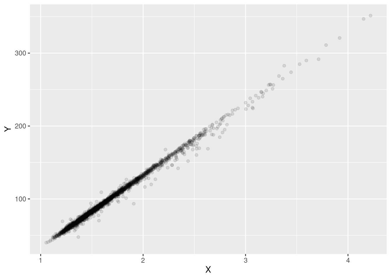
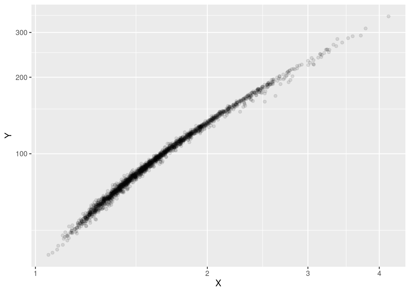
Let’s start by looking at a scatter plot (Figure 1). This suggests a strong linear relation between $X$ and $Y$ . Plotting the point with transparency reveals that the density of the observations depends on the value. This is confirmed by the skewed distribution shown in Figure 2. This is something we have to keep in mind.

ggplot(dataset, aes(x = X, y = Y)) + geom_point(alpha = 0.1)

dataset %>%
  select(-ID) %>%
  gather("Variable", "Value") %>%
  ggplot(aes(x = Value)) + geom_density() +
  facet_wrap(~Variable, scales = "free")

The mathematical equation of the random slope model is given in Equation 1. It contains a fixed intercept and fixed slope along $X$ and a random intercept and random slope along $X$ for each $I D$ . The random intercept $b_{0 i}$ and random slope stem $b_{1 i}$ from a bivariate normal distribution.

$\begin{matrix} (1) & Y \sim N (μ, σ_{ε}^{2}) \end{matrix}$ $μ = β_{0} + β_{1} X + b_{0 i} + b_{1 i} X$ $b \sim N (0, Σ^{2})$

The number of groups and the number of observations per group are two important things to check before running a mixed model. Figure 3 indicates that there are plenty of groups but a large number of groups have only one or just a few observations. This is often problematic in combination with a random slope. Let’s see what the random slope actually does by cutting some corners and simplifying the mixed model into a set of hierarchical linear models. We have one linear model ‘FE’ that fits the response using only the fixed effects. For each group we fit another linear model on the residuals of model ‘FE’. So when there are only two observations in a group, the random slope model fits a straight line through only two points… To make things even worse, many groups have quite a small span (Figure 4). Image the worst case were a group has only two observations, both have extreme and opposite residuals from model ‘FE’ and their span is small. The result will be an extreme random slope…

dataset %>%
  count(ID) %>%
  ggplot(aes(x = n)) + geom_histogram(binwidth = 1)

Figure 3: Histogram of the number of observations per group

dataset %>%
  group_by(ID) %>%
  summarise(
    span = max(X) - min(X),
    n = n()
  ) %>%
  filter(n > 1) %>%
  ggplot(aes(x = span)) + geom_density()

Figure 4: Density of the span (difference between min and max) for all groups with at least 2 observations

Original model

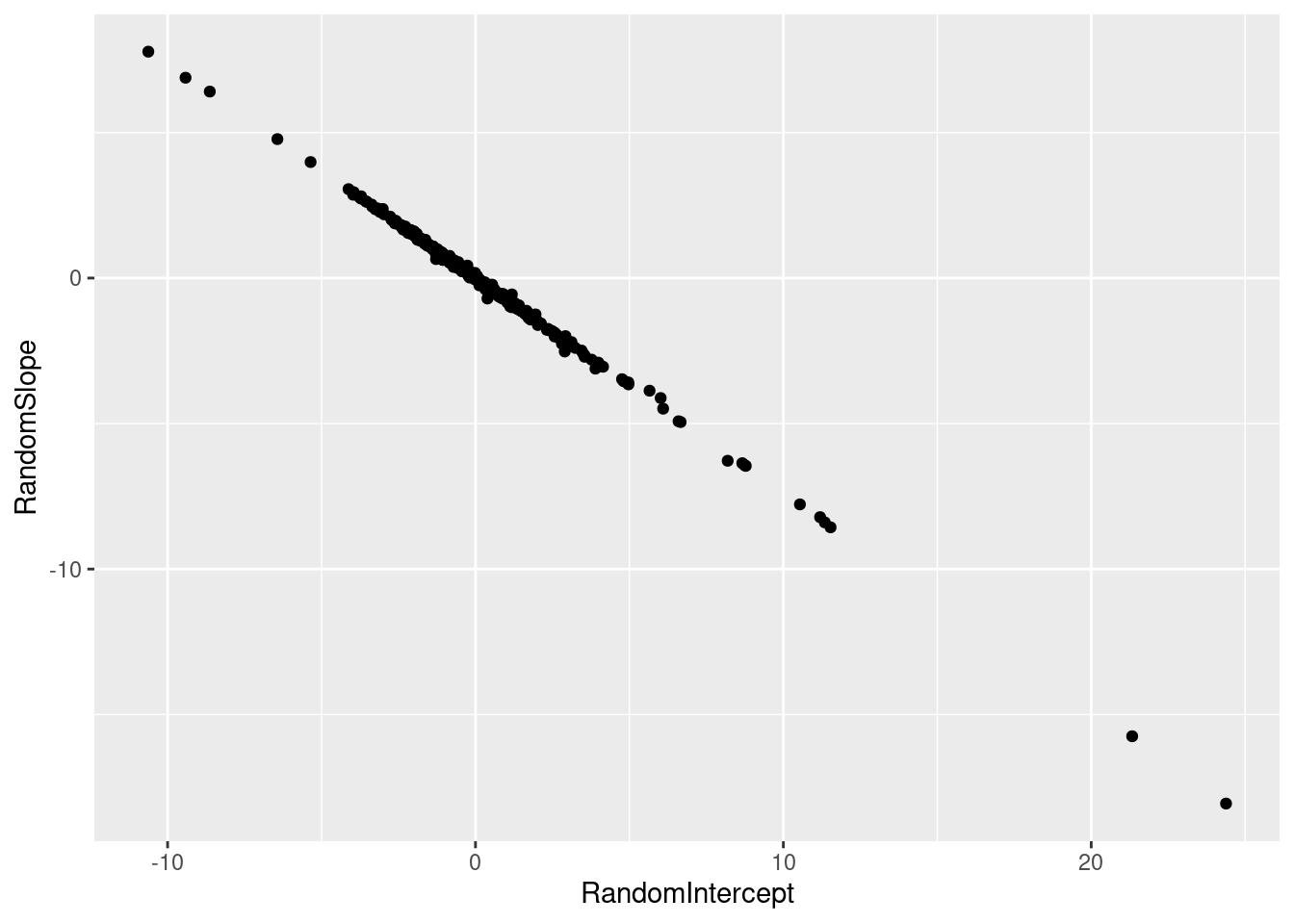
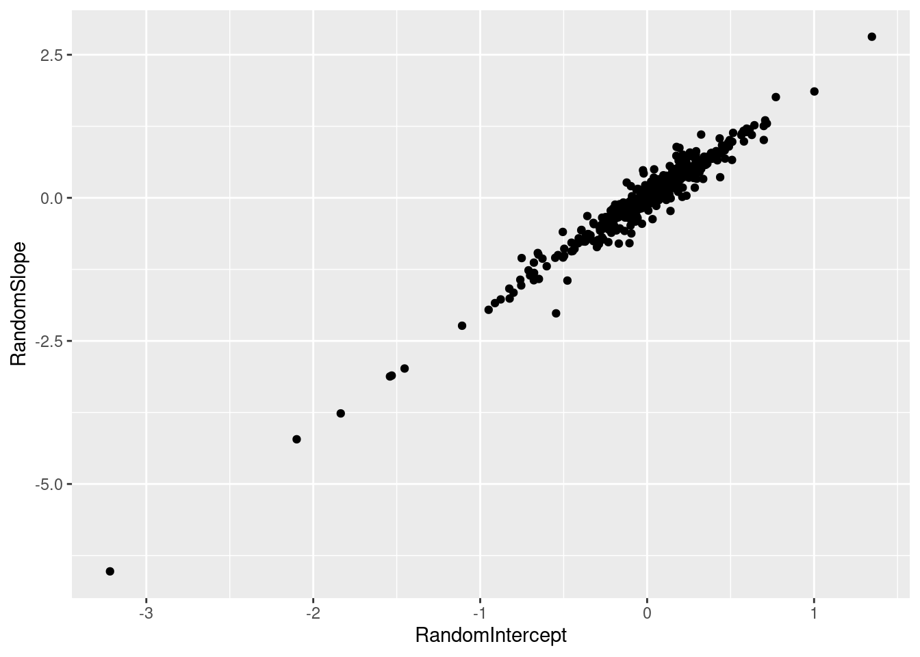
First we fit the original model. Notice the perfect negative correlation between the random intercept and the random slope. This triggered, rightly, an alarm with the researcher. The perfect correlation is clear when looking at a scatter plot of the random intercepts and random slopes (Figure 5). Figure 6 show the nine most extreme random slopes. The Y-axis displays the difference between the observed $Y$ and the model fit using only the fixed effects ( $β_{0} + β_{1} X$ ). Note that the random slopes are not as strong as what we would expect from the naive hierarchical model we described above. Mixed models apply shrinkage to the coefficients of the random effects, making them less extreme.

model <- lmer(Y ~ X + (X | ID), data = dataset)
summary(model)

Linear mixed model fit by REML ['lmerMod']
Formula: Y ~ X + (X | ID)
   Data: dataset

REML criterion at convergence: 10753.1

Scaled residuals: 
    Min      1Q  Median      3Q     Max 
-8.6576 -0.3511  0.0692  0.4535  6.5774 

Random effects:
 Groups   Name        Variance Std.Dev. Corr 
 ID       (Intercept) 21.050   4.588         
          X           11.102   3.332    -1.00
 Residual              6.124   2.475         
Number of obs: 2234, groups:  ID, 601

Fixed effects:
            Estimate Std. Error t value
(Intercept) -64.3591     0.4219  -152.6
X            98.0603     0.2783   352.4

Correlation of Fixed Effects:
  (Intr)
X -0.986

rf <- ranef(model)$ID %>%
  select(RandomIntercept = 1, RandomSlope = 2) %>%
  rownames_to_column("ID") %>%
  mutate(ID = as.integer(ID))
ggplot(rf, aes(x = RandomIntercept, y = RandomSlope)) + geom_point()

Figure 5: Scatterplot of the random intercepts and random slopes.

dataset <- dataset %>%
  mutate(
    Resid = resid(model),
    Fixed = predict(model, re.form = ~0)
  )
rf %>%
  arrange(desc(abs(RandomSlope))) %>%
  slice(1:9) %>%
  inner_join(dataset, by = "ID") %>%
  ggplot(aes(x = X, y = Y - Fixed)) +
  geom_point() +
  geom_hline(yintercept = 0, linetype = 2) +
  geom_abline(aes(intercept = RandomIntercept, slope = RandomSlope)) +
  facet_wrap(~ID)

Figure 6: Illustration of the most extreme random slopes.

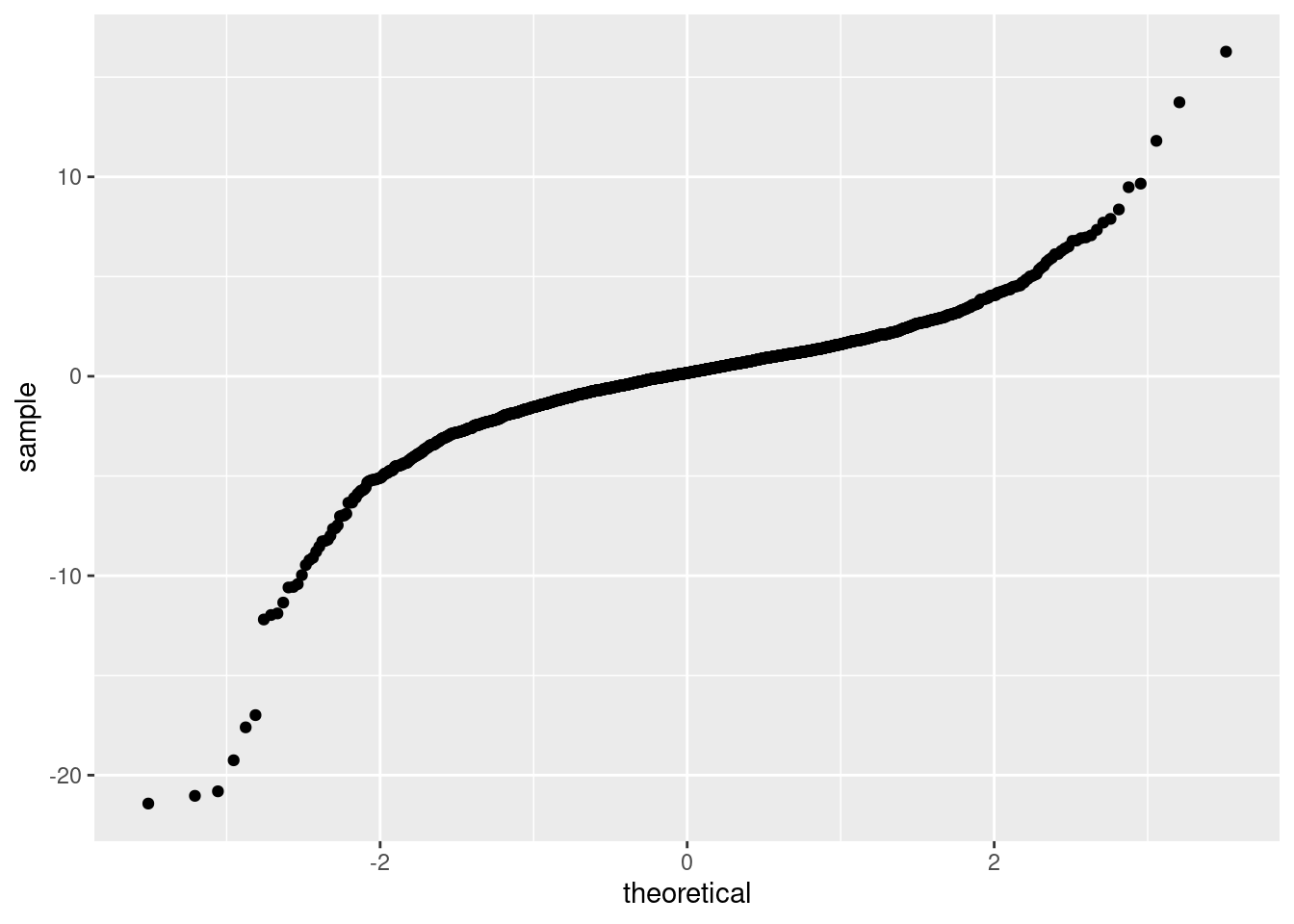
Until now, we focused mainly on the random effects. Another thing one must check are the residuals. The QQ-plot (Figure 7) indicates that several observations have quite strong residuals. Those should be checked by an expert with domain knowledge on the data. I recommend to start by looking at the top 20 observations with the most extreme residuals. Question the data for these observations: e.g. was the measurement correct, was the data entry correct, … When the data turns out to be OK, question it’s relevance for the model (e.g. is the observation a special case) and question the model itself (e.g. are missing something important in the model, does the model makes sense). Refit the model after the data cleaning and repeat the process until you are happy with both the model and the data.

ggplot(dataset, aes(sample = Resid)) + stat_qq()

Potential solutions

Removing questionable observations

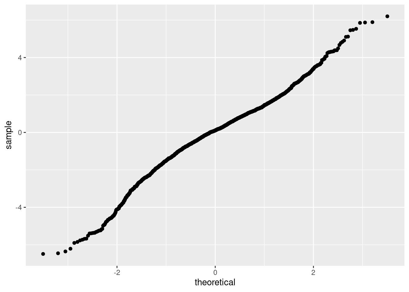
Here we demonstrate what happens in case all observations with strong residuals turn out to be questionable and are removed from the data. Note that we do not recommend to simply remove all observation with strong residuals. Instead have a domain expert scrutinise each observation and remove only those observations which are plain wrong or not relevant. This is something I can’t do in this case because I don’t have the required domain knowledge. For demonstration purposes I’ve removed all observations who’s residuals are outside the (0.5%, 99.5%) quantile of the theoretical distribution of the residuals. The QQ-plot (fig. @ref(fig:qq-cleaned)) now looks OK, but we still have perfect correlation among the random effects.

dataset_cleaned <- dataset %>%
  filter(abs(Resid) < qnorm(0.995, mean = 0, sd = sigma(model)))
model_cleaned <- lmer(Y ~ X + (X | ID), data = dataset_cleaned)
summary(model_cleaned)

Linear mixed model fit by REML ['lmerMod']
Formula: Y ~ X + (X | ID)
   Data: dataset_cleaned

REML criterion at convergence: 9182.5

Scaled residuals: 
    Min      1Q  Median      3Q     Max 
-3.6053 -0.4946  0.0577  0.5772  3.4444 

Random effects:
 Groups   Name        Variance Std.Dev. Corr 
 ID       (Intercept) 20.973   4.580         
          X            9.500   3.082    -1.00
 Residual              3.241   1.800         
Number of obs: 2188, groups:  ID, 598

Fixed effects:
            Estimate Std. Error t value
(Intercept) -64.6873     0.3471  -186.3
X            98.3516     0.2257   435.7

Correlation of Fixed Effects:
  (Intr)
X -0.989

dataset_cleaned %>%
  mutate(Resid = resid(model_cleaned)) %>%
  ggplot(aes(sample = Resid)) + stat_qq()

Figure 8: QQ-plot for the original model on the cleaned dataset.

Centring and scaling

Another thing that often can help is centring and scaling the data. In this case we centre to a zero mean and scale to a standard deviation of 1. Personally I prefer to centre to some meaningful value in the data. E.g. when the variable is the year of the observation I would centre to the first year, last year or some other important year within the dataset. This makes the interpretation of the model parameters easier. I usually scale variables by some power of 10 again because of the interpretation of the parameters.

We will keep using the cleaned dataset so that the problematic observation don’t interfere with the effect of centring and scaling. Scaling improves the correlation between the random intercept and the random slope. It is no longer a perfect correlation but still quite strong (Figure 9). Note that the sign of the correlation has changed. Although we removed the questionable observations, there are still some groups of observations with quite strong deviations from the fixed effects part from the model (Figure 10).

dataset_cleaned <- dataset_cleaned %>%
  mutate(
    Xcs = scale(X, center = TRUE, scale = TRUE)
  )
model_centered <- lmer(Y ~ X + (Xcs | ID), data = dataset_cleaned)
summary(model_centered)

Linear mixed model fit by REML ['lmerMod']
Formula: Y ~ X + (Xcs | ID)
   Data: dataset_cleaned

REML criterion at convergence: 9182.5

Scaled residuals: 
    Min      1Q  Median      3Q     Max 
-3.6053 -0.4946  0.0577  0.5772  3.4444 

Random effects:
 Groups   Name        Variance Std.Dev. Corr
 ID       (Intercept) 0.3996   0.6322       
          Xcs         1.4161   1.1900   0.88
 Residual             3.2413   1.8004       
Number of obs: 2188, groups:  ID, 598

Fixed effects:
            Estimate Std. Error t value
(Intercept) -64.6873     0.3471  -186.4
X            98.3516     0.2257   435.7

Correlation of Fixed Effects:
  (Intr)
X -0.989

rf <- ranef(model_centered)$ID %>%
  select(RandomIntercept = 1, RandomSlope = 2) %>%
  rownames_to_column("ID") %>%
  mutate(ID = as.integer(ID))
ggplot(rf, aes(x = RandomIntercept, y = RandomSlope)) + geom_point()

Figure 9: Scatterplot of the random intercepts and random slopes after centering and scaling.

dataset_cleaned <- dataset_cleaned %>%
  mutate(
    Resid = resid(model_centered),
    Fixed = predict(model_centered, re.form = ~0)
  )
rf %>%
  arrange(desc(abs(RandomSlope))) %>%
  slice(1:9) %>%
  inner_join(dataset_cleaned, by = "ID") %>%
  ggplot(aes(x = X, y = Y - Fixed)) +
  geom_point() +
  geom_hline(yintercept = 0, linetype = 2) +
  geom_abline(aes(intercept = RandomIntercept, slope = RandomSlope)) +
  facet_wrap(~ID)

Figure 10: Illustration of the most extreme random slopes after centering and scaling.

Simplifying the model

Based on Figure 3 and Figure 4 we already concluded that a random slope might be pushing it for this data set. So an obvious solution is to remove the random slope and only keep the random intercept. Though there still are quite a large number of groups with only one observation (Figure 3), this is often less problematic in case you have plenty of groups with multiple observations. Note that the variance of the random intercept of this model is much smaller than in the previous models. The random intercept model is not as good as the random slope model in terms of AIC, but this comparison is a bit pointless since the random slope model is not trustworthy.

model_simple <- lmer(Y ~ X + (1 | ID), data = dataset_cleaned)
summary(model_simple)

Linear mixed model fit by REML ['lmerMod']
Formula: Y ~ X + (1 | ID)
   Data: dataset_cleaned

REML criterion at convergence: 9593.6

Scaled residuals: 
    Min      1Q  Median      3Q     Max 
-6.2261 -0.4503  0.0682  0.5238  6.0184 

Random effects:
 Groups   Name        Variance Std.Dev.
 ID       (Intercept) 1.897    1.377   
 Residual             3.688    1.921   
Number of obs: 2188, groups:  ID, 598

Fixed effects:
            Estimate Std. Error t value
(Intercept) -64.1588     0.2736  -234.5
X            97.9788     0.1572   623.2

Correlation of Fixed Effects:
  (Intr)
X -0.959

anova(model_centered, model_simple)

refitting model(s) with ML (instead of REML)

Data: dataset_cleaned
Models:
model_simple: Y ~ X + (1 | ID)
model_centered: Y ~ X + (Xcs | ID)
               npar    AIC    BIC  logLik deviance  Chisq Df Pr(>Chisq)    
model_simple      4 9596.4 9619.2 -4794.2   9588.4                         
model_centered    6 9189.2 9223.3 -4588.6   9177.2 411.22  2  < 2.2e-16 ***
---
Signif. codes:  0 '***' 0.001 '**' 0.01 '*' 0.05 '.' 0.1 ' ' 1

Transformations

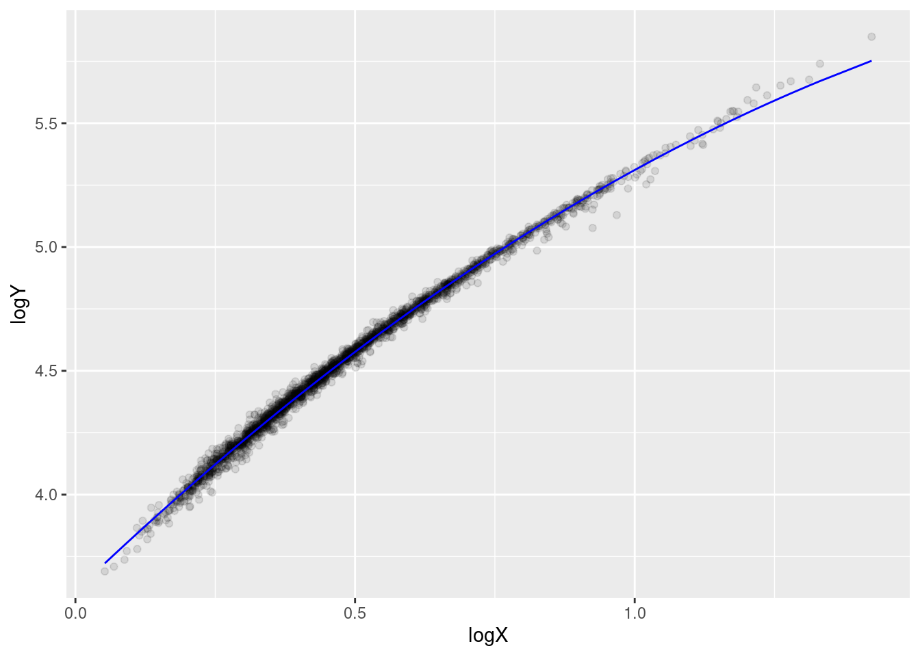
Figure 2 indicated that the distribution of both $X$ and $Y$ is quite skewed. A $l o g$ -transformation reduces the skewness (Figure 11) and reveals a quadratic relation between $\log (X)$ and $\log (Y)$ (Figure 12).

dataset_cleaned %>%
  select(X, Y) %>%
  gather("Variable", "Value") %>%
  ggplot(aes(x = log(Value))) + geom_density() +
  facet_wrap(~Variable, scales = "free")

Figure 11: Density of $X$ and $Y$ after log-transformation

ggplot(dataset_cleaned, aes(x = X, y = Y)) + geom_point(alpha = 0.1) +
  coord_trans(x = "log", y = "log")

Figure 12: Scatterplot after log-transformation.

This might be a relevant transformation, but it needs to be checked by a domain expert because this random slope model Equation 2 expresses a different relation between $X$ and $Y$ . The fixed part of model Equation 2 becomes $Y \sim e^{γ_{0}} X^{γ_{1}}$ after back transformation.

$\begin{matrix} (2) & \log (Y) \sim N (η, σ_{ε}^{2}) \end{matrix}$ $η = γ_{0} + γ_{1} \log (X) + c_{0 i}$ $c \sim N (0, σ^{2})$

dataset_cleaned <- dataset_cleaned %>%
  mutate(logY = log(Y), logX = log(X))
model_log <- lmer(logY ~ logX + (1 | ID), data = dataset_cleaned)
summary(model_log)

Linear mixed model fit by REML ['lmerMod']
Formula: logY ~ logX + (1 | ID)
   Data: dataset_cleaned

REML criterion at convergence: -8723.6

Scaled residuals: 
    Min      1Q  Median      3Q     Max 
-6.3306 -0.4654  0.1075  0.5517  2.8275 

Random effects:
 Groups   Name        Variance  Std.Dev.
 ID       (Intercept) 0.0006140 0.02478 
 Residual             0.0007947 0.02819 
Number of obs: 2188, groups:  ID, 598

Fixed effects:
            Estimate Std. Error t value
(Intercept) 3.747007   0.002623  1428.6
logX        1.612781   0.004681   344.5

Correlation of Fixed Effects:
     (Intr)
logX -0.871

A quadratic fixed effect of $\log (X)$ improves the model a lot. The resulting fit is given in Figure 13.

model_log2 <- lmer(logY ~ poly(logX, 2) + (1 | ID), data = dataset_cleaned)
anova(model_log, model_log2)

refitting model(s) with ML (instead of REML)

Data: dataset_cleaned
Models:
model_log: logY ~ logX + (1 | ID)
model_log2: logY ~ poly(logX, 2) + (1 | ID)
           npar    AIC      BIC logLik deviance  Chisq Df Pr(>Chisq)    
model_log     4  -8736  -8713.2 4372.0    -8744                         
model_log2    5 -10434 -10406.0 5222.2   -10444 1700.4  1  < 2.2e-16 ***
---
Signif. codes:  0 '***' 0.001 '**' 0.01 '*' 0.05 '.' 0.1 ' ' 1

summary(model_log2)

Linear mixed model fit by REML ['lmerMod']
Formula: logY ~ poly(logX, 2) + (1 | ID)
   Data: dataset_cleaned

REML criterion at convergence: -10420.7

Scaled residuals: 
    Min      1Q  Median      3Q     Max 
-4.6171 -0.4938  0.0662  0.5359  4.1296 

Random effects:
 Groups   Name        Variance  Std.Dev.
 ID       (Intercept) 9.311e-05 0.00965 
 Residual             4.329e-04 0.02081 
Number of obs: 2188, groups:  ID, 598

Fixed effects:
                 Estimate Std. Error t value
(Intercept)     4.5311687  0.0006646 6817.57
poly(logX, 2)1 15.8221541  0.0273352  578.82
poly(logX, 2)2 -1.3249513  0.0250247  -52.95

Correlation of Fixed Effects:
            (Intr) p(X,2)1
ply(lgX,2)1 -0.007        
ply(lgX,2)2 -0.029 -0.065

dataset_cleaned <- dataset_cleaned %>%
  mutate(Fixed = predict(model_log2, re.form = ~0))
ggplot(dataset_cleaned, aes(x = logX, y = logY)) +
  geom_point(alpha = 0.1) +
  geom_line(aes(y = Fixed), colour = "blue")

Figure 13: Predictions for the fixed effect of the quadratic model on $\log (X)$

Conclusions

First of all the data set needs to be checked for potential errors in the data.
The current design of the data does not support a random slope model.
A transformation of the variables might be relevant.

Session info

sessioninfo::session_info()

─ Session info ───────────────────────────────────────────────────────────────
 setting  value
 version  R version 4.3.1 (2023-06-16)
 os       Ubuntu 22.04.3 LTS
 system   x86_64, linux-gnu
 ui       X11
 language nl_BE:nl
 collate  nl_BE.UTF-8
 ctype    nl_BE.UTF-8
 tz       Europe/Brussels
 date     2023-08-30
 pandoc   3.1.1 @ /usr/lib/rstudio/resources/app/bin/quarto/bin/tools/ (via rmarkdown)

─ Packages ───────────────────────────────────────────────────────────────────
 package     * version    date (UTC) lib source
 bit           4.0.5      2022-11-15 [1] CRAN (R 4.3.0)
 bit64         4.0.5      2020-08-30 [1] CRAN (R 4.3.0)
 boot          1.3-28.1   2022-11-22 [1] CRAN (R 4.3.0)
 cli           3.6.1      2023-03-23 [1] CRAN (R 4.3.0)
 colorspace    2.1-0      2023-01-23 [1] CRAN (R 4.3.0)
 crayon        1.5.2      2022-09-29 [1] CRAN (R 4.3.0)
 digest        0.6.32     2023-06-26 [1] CRAN (R 4.3.1)
 dplyr       * 1.1.2      2023-04-20 [1] CRAN (R 4.3.0)
 evaluate      0.21       2023-05-05 [1] CRAN (R 4.3.0)
 fansi         1.0.4      2023-01-22 [1] CRAN (R 4.3.0)
 farver        2.1.1      2022-07-06 [1] CRAN (R 4.3.0)
 fastmap       1.1.1      2023-02-24 [1] CRAN (R 4.3.0)
 forcats     * 1.0.0      2023-01-29 [1] CRAN (R 4.3.0)
 generics      0.1.3      2022-07-05 [1] CRAN (R 4.3.0)
 ggplot2     * 3.4.2      2023-04-03 [1] CRAN (R 4.3.0)
 glue          1.6.2      2022-02-24 [1] CRAN (R 4.3.0)
 gtable        0.3.3      2023-03-21 [1] CRAN (R 4.3.0)
 hms           1.1.3      2023-03-21 [1] CRAN (R 4.3.0)
 htmltools     0.5.5      2023-03-23 [1] CRAN (R 4.3.0)
 htmlwidgets   1.6.2      2023-03-17 [1] CRAN (R 4.3.0)
 jsonlite      1.8.7      2023-06-29 [1] CRAN (R 4.3.1)
 knitr         1.43       2023-05-25 [1] CRAN (R 4.3.0)
 labeling      0.4.2      2020-10-20 [1] CRAN (R 4.3.0)
 lattice       0.21-8     2023-04-05 [4] CRAN (R 4.3.0)
 lifecycle     1.0.3      2022-10-07 [1] CRAN (R 4.3.0)
 lme4        * 1.1-34     2023-07-04 [1] CRAN (R 4.3.1)
 lubridate   * 1.9.2.9000 2023-05-15 [1] https://inbo.r-universe.dev (R 4.3.0)
 magrittr      2.0.3      2022-03-30 [1] CRAN (R 4.3.0)
 MASS          7.3-60     2023-05-04 [4] CRAN (R 4.3.1)
 Matrix      * 1.5-4.1    2023-05-18 [1] CRAN (R 4.3.0)
 minqa         1.2.5      2022-10-19 [1] CRAN (R 4.3.0)
 munsell       0.5.0      2018-06-12 [1] CRAN (R 4.3.0)
 nlme          3.1-162    2023-01-31 [1] CRAN (R 4.3.0)
 nloptr        2.0.3      2022-05-26 [1] CRAN (R 4.3.0)
 pillar        1.9.0      2023-03-22 [1] CRAN (R 4.3.0)
 pkgconfig     2.0.3      2019-09-22 [1] CRAN (R 4.3.0)
 purrr       * 1.0.1      2023-01-10 [1] CRAN (R 4.3.0)
 R6            2.5.1      2021-08-19 [1] CRAN (R 4.3.0)
 Rcpp          1.0.10     2023-01-22 [1] CRAN (R 4.3.0)
 readr       * 2.1.4      2023-02-10 [1] CRAN (R 4.3.0)
 rlang         1.1.1      2023-04-28 [1] CRAN (R 4.3.0)
 rmarkdown     2.23       2023-07-01 [1] CRAN (R 4.3.1)
 rstudioapi    0.14       2022-08-22 [1] CRAN (R 4.3.0)
 scales        1.2.1      2022-08-20 [1] CRAN (R 4.3.0)
 sessioninfo   1.2.2      2021-12-06 [1] CRAN (R 4.3.0)
 stringi       1.7.12     2023-01-11 [1] CRAN (R 4.3.0)
 stringr     * 1.5.0      2022-12-02 [1] CRAN (R 4.3.0)
 tibble      * 3.2.1      2023-03-20 [1] CRAN (R 4.3.0)
 tidyr       * 1.3.0      2023-01-24 [1] CRAN (R 4.3.0)
 tidyselect    1.2.0      2022-10-10 [1] CRAN (R 4.3.0)
 tidyverse   * 2.0.0      2023-02-22 [1] CRAN (R 4.3.0)
 timechange    0.2.0      2023-01-11 [1] CRAN (R 4.3.0)
 tzdb          0.4.0      2023-05-12 [1] CRAN (R 4.3.0)
 utf8          1.2.3      2023-01-31 [1] CRAN (R 4.3.0)
 vctrs         0.6.3      2023-06-14 [1] CRAN (R 4.3.0)
 vroom         1.6.3      2023-04-28 [1] CRAN (R 4.3.0)
 withr         2.5.0      2022-03-03 [1] CRAN (R 4.3.0)
 xfun          0.39       2023-04-20 [1] CRAN (R 4.3.0)
 yaml          2.3.7      2023-01-23 [1] CRAN (R 4.3.0)

 [1] /home/thierry/R/x86_64-pc-linux-gnu-library/4.3
 [2] /usr/local/lib/R/site-library
 [3] /usr/lib/R/site-library
 [4] /usr/lib/R/library

──────────────────────────────────────────────────────────────────────────────